easy beginning#
Generate artificial signals#
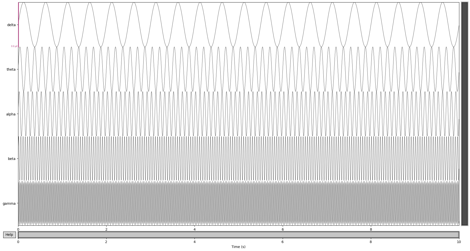
We generate five-channel signals with special frequency bands. The five channels have high amplitude in the following frequency bands: Delta (1-4 Hz), Theta (4-8 Hz), Alpha (8-13 Hz), Beta (13-30 Hz), and Gamma (30-50 Hz).
Generate time signals#
[2]:
sfreq = 256
t = np.arange(0, 10, 1/sfreq)
delta = np.sin(2 * np.pi * 2 * t)  # Delta (1-4 Hz)
theta = np.sin(2 * np.pi * 6 * t)  # Theta (4-8 Hz)
alpha = np.sin(2 * np.pi * 10 * t)  # Alpha (8-13 Hz)
beta = np.sin(2 * np.pi * 20 * t)  # Beta (13-30 Hz)
gamma = np.sin(2 * np.pi * 40 * t)  # Gamma (30-100 Hz
data = np.vstack([delta, theta, alpha, beta, gamma])
print(data.shape)
(5, 2560)
Place the signal into MNE’s raw structure.#
[3]:
info = mne.create_info(ch_names=['delta', 'theta', 'alpha', 'beta', 'gamma'], sfreq=sfreq, ch_types='eeg')
raw = mne.io.RawArray(data, info)
Creating RawArray with float64 data, n_channels=5, n_times=2560
    Range : 0 ... 2559 =      0.000 ...     9.996 secs
Ready.
plot signals#
[4]:
# plot time series
raw.plot(n_channels=5, scalings='auto', title='Time Domain Signals', show=False)
Using matplotlib as 2D backend.
[4]:

[5]:
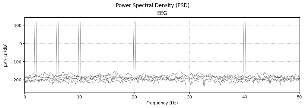
# plot psd
fig = raw.plot_psd(fmax=50, n_fft=2048, show=False)
fig.suptitle('Power Spectral Density (PSD)')
plt.show()
NOTE: plot_psd() is a legacy function. New code should use .compute_psd().plot().
Effective window size : 8.000 (s)
C:\Users\15956\AppData\Local\Temp\ipykernel_34216\3419607408.py:2: RuntimeWarning: Channel locations not available. Disabling spatial colors.
  fig = raw.plot_psd(fmax=50, n_fft=2048, show=False)
calculate feature by scuteegfe#
‘pow_freq_bands’ is in mne-feature function. We introduce its usage in scuteegfe, which is the same as mne-feature package. selected_funcs is a list contained all func str that you need. funcs_params is a dict for your funcs_params.
calculate#
data shape (n_epochs, n_channels, n_times)
[6]:
print(data[None,:].shape)
(1, 5, 2560)
The function in API “compute_pow_freq_bands”, correlated selected_funcs is [‘pow_freq_bands’]. This is consistent with the MNE-Feature package.
[ ]:
fea = Feature(data[None,:], sfreq=sfreq, selected_funcs=['pow_freq_bands'],
               funcs_params={"pow_freq_bands__freq_bands":np.array([[1,4],[4,8],[8,13],[18,22],[30,50]]),
                            "pow_freq_bands__normalize": False})
return description#
[8]:
print(fea)
1(epochs) x 5(channels) x 5(features)
feature names: ['pow_freq_bands0' 'pow_freq_bands1' 'pow_freq_bands2' 'pow_freq_bands3'
 'pow_freq_bands4']
[9]:
n_epochs, n_channels, n_features = fea.features.shape
print(n_epochs, n_channels, n_features)
1 5 5
[10]:
df = pd.DataFrame(np.squeeze(fea.features), columns=fea.feature_names)
df.index = [f'Channel {i+1}' for i in range(n_channels)]
df
[10]:
| pow_freq_bands0 | pow_freq_bands1 | pow_freq_bands2 | pow_freq_bands3 | pow_freq_bands4 | |
|---|---|---|---|---|---|
| Channel 1 | 5.000000e-01 | 3.331320e-32 | 1.434390e-32 | 2.252499e-31 | 2.568837e-31 |
| Channel 2 | 7.581579e-32 | 5.000000e-01 | 1.339228e-31 | 5.540426e-31 | 2.085246e-30 |
| Channel 3 | 2.337820e-29 | 5.342350e-31 | 5.000000e-01 | 2.548555e-29 | 1.695981e-29 |
| Channel 4 | 3.193826e-29 | 8.265879e-29 | 9.076266e-29 | 5.000000e-01 | 1.496328e-28 |
| Channel 5 | 1.648561e-29 | 8.346900e-29 | 1.349165e-29 | 2.121023e-29 | 5.000000e-01 |